Divisive Normalization – a Universal Concept for Adaptive Dynamics and Function of Cortical Circuits

Neural computation is highly flexible and adjusts the spatio-temporal context of external stimuli and to the current behavioral task. This flexibility is an important aspect why squishy brains are under the rapidly changing conditions in daily life still superior to machines. Divisive normalization is a fundamental concept realizing an adaptive dynamics which has interesting functional consequences. For example, it can enhance changes in the sensory input: Think of a tiger suddenly leaping from its hiding place: can your brain detect this change in a natural scene in time, or will you be a delicious meal just a few moments later? Another benefit of divisive normalization is the increase of the operating regime of a neural circuit, making sensitivity to changes more independent from average activation levels. Starting from understanding and managing the basic concepts of divisive normalization and its modeling, this Advanced Studies project can be extended into several directions depending on student interests, and it links to on-going research in our lab. Some tasks described below should be done by all the students, more advanced tasks can be split among the group (marked with ADV)

1. Make a model with divisive inhibition

The basic network to be investigated consists of an excitatory unit, which receives divisive input from an inhibitory unit (see Figure). The units have activation levels $A_e$ and $A_i$. Its dynamics should be described by two coupled differential equations (DEQs) which have the general form $\tau dA/dt = -A+g(I)$, and where $\tau$ is a time constant, and $g$ piecewise linear gain functions on the input $I$. We will name this model the Divisive Inhibition on Excitation-model, short DivInE-model. With the right set of parameters, this model is capable to reproduce physiological data from monkey area MT [3].

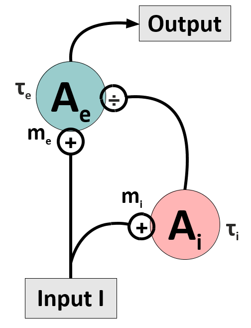
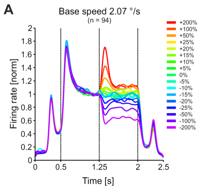
In particular, when subjected to abrupt changes in the input $I$, the circuit can respond with a huge overshoot or undershoot in its firing rate before settling into a stationary state. These dynamics are called ‘transient responses’, and they can nicely be seen in the graph on the right hand side (from [3]).

a.

Write down the system of two coupled DEQs. For $t \longrightarrow \infty$, the excitatory unit shall give an output similar to Eq. (2) in reference [1] (with corresponding renaming of variables, of course).

2. Implement the DivInE-model on your computer

For every following numerical investigation, it is necessary that you can simulate this simple circuit in a computer. Simulations also help you to play around with parameters and to understand ‘intuitively’ how the circuit works.

a.

Write a function which integrates the two coupled DEQs numerically using the Euler scheme.

b.

Test your code by subjecting your neural circuit to a step current. Plot the responses of the two units into one graph.

c.

Can you generate responses which are similar to the physiological data shown above? How do you have to choose the parameters, in particular the time constants of the model?

3. Analyze the transfer characteristics of the DivInE-model

When looking at the physiological data, it seems as if the DivInE-model ‘likes’ fast changes more than strong input currents. We can investigate this property systematically by computing the transfer characteristics of the model, i.e. how well changes on a particular time scale (frequency) are transmitted by the circuit.

a.

Generate a white noise signal $I(t)$ and use it as an input to your circuit.

b.

Record the circuits’ responses (both for $A_e(t)$ and $A_i(t)$) and compute the amplitude spectrum of the input signal $I(t)$, and of the neural output signals $A_e(t)$ and $A_i(t)$.

c.

Accumulate the amplitude spectra over many different realizations of the input $I(t)$ and plot them into one single graph.

d.

Interpret your results! How can you describe what the circuit ‘does’ to an arbitrary input?

e.

Set the time constants in the model in relation to the amplitude spectra.

f.

If you are ambitious, compute the amplitude spectrum for the inhibitory unit analytically and compare it to the numerical spectrum.

ADV 4. Analyze the DivInE-model

For understanding the behavior of the model, and for being able to efficiently fit the model to physiological data, it is useful to analyze the neural dynamics analytically as far as possible.

a.

Assume the external input is always larger than zero, $I(t)>0$. How can you simplify the DEQs and get rid of the non-linearity?

b.

What are the fixed points of the two DEQs for a constant input current? Are these fixed points stable?

c.

Compute the maximum firing rate $A_e^{max}$ the excitatory unit can achieve.

d.

Assume the input is a step function, $I(t)=I_0$ for $t<0$ and $I(t)=I_1$ for $t\geq0$. Solve the DEQ for the inhibitory unit.

e.

Insert the solution of the DEQ for the inhibitory unit into the DEQ for the excitatory unit. You have now simplified the system to only one DEQ - super!

ADV 5. Fit the DivInE-model to physiological data

How well can our circuit quantitatively fit physiological data? Let’s find out! We provide you with population data from macaque area MT, and your task will be to fit the model to the data.

a.

We provide you with a file in which we stored eight neural response functions to a stimulus change (acceleration and deceleration of a moving grating). The stimulus change happened at time $t=0$, see the time axis stored in the same file.

b.

Fit the model output to the physiological response, as best as possible. In the following, we will give you some tips and tricks how this could be done:

• From the analysis performed above, you know that for an input step (which is comparable to the experimental situation here), you only need one DEQ.
• Now it is a good idea to get rid of as many free parameters as possible: From the physiological traces you can see that before and after the stimulus change, the activity settles into a stationary state, say $A_e^0$ and $A_e^1$. You can extract these values directly from the experimental data.
• You can now rewrite the DEQ by using the new parameters $A_e^0$ and $A_e^1$, and the maximum activation $A_e^{max}$, to get rid of the parameters $m_e, m_i, I$ and $B$. This leaves you with only three parameters to fit.
• For performing the fit, you have to define an objective function which evaluates how close your fit to the original data is. For example, the mean quadratic distance between model and physiological traces.
• Inform yourself about different methods for optimizing an objective function with respect to a set of free parameters. For example, grid search or (stochastic) gradient descent. Understand also the caveats of these methods!
• Take care of delays in the physiological response, the stimulus signal needs some time to travel to area MT!

ADV 6. The DivInE-model and attention

Attention serves to enhance neural responses to selected stimuli relative to representations of unattended stimuli. Hereby divisive inhibition seems to play a central role as a control mechanism – several studies in our lab are currently investigating corresponding effects. If you are interested in learning more about these studies, and extend your project in that direction, we offer you two possibilites (talk to your tutor for receiving detailed guidance and instructions). Ref. [2] tells you more about attention can be introduced in your model.

a.

Divisive normalization enhances transients [4]: How does attention enhance transient responses? You can investigate this numerically in your model, and compare it to the MT data we provide for you. We recommend you to have a look at three typical features of a neural response to a current step: the change in sustained response, the relative peak response, and the initial increase of the transient. What do you observe? How would you investigate corresponding effects systematically?

b.

Divisive normalization increases working range of selective attention [5]: When two stimuli are in the receptive field of a cortical neuron, and one of those stimuli is attended, the cell responds as if only the attended stimulus was present. Most probably, the brain achieves this effect by generating a small rate advantage in the presynaptic population driven by the attended stimulus, which is amplified by recurrent processes for effectively routing only the attended signal to postsynaptic circuits. However, this mechanism is challenged if the attended stimulus provides a much weaker input drive than the non-attended stimulus. How could selective processing still work? One potential answer is that divisive normalization increases the ‘working range’ over which a rate advantage for the attended stimulus is created. You can easily investigate this effect by simulating two coupled DivInE-circuits.

Literature

[1] Carandini, M., \& Heeger, D. J. (2011). Normalization as a canonical neural computation. Nat Rev Neurosci. ; 13(1): 51–62. doi:10.1038/nrn3136.

[2] Reynolds, J. H., \& Heeger, D. J. (2009). The normalization model of attention. Neuron, 61(2), 168–185. https://doi.org/10.1016/j.neuron.2009.01.002

[3] Traschütz A., Kreiter A. K., \& Wegener D. (2015). Transient activity in monkey area MT represents speed changes and is correlated with human behavioral performance. J Neurophysiol. 113: 890-903.

[4] Ernst, U., Chen, X., Bohnenkamp, L., Galashan, F. O., \& Wegener, D. (2020). A simple canonical circuitry for non-stationary normalization by inhibition to explain and predict change detection in monkey area MT. In preparation.

[5] Rausch, L.-P., Schünemann, M., Drebitz, E., Harnack, D., Kreiter, A. K., \& Ernst, U. (2020) Strong attentional modulation of V1/V2 activity implements a robust, contrast-invariant control mechanism for selective information processing. In preparation.

The source code is Open Source and can be found on GitHub.