FFT
The goal
Fouriert transformations are an important part of data analysis.
Questions to David Rotermund
Numpy vs scipy
pip install scipy
Numpy says itself:
The SciPy module scipy.fft is a more comprehensive superset of numpy.fft, which includes only a basic set of routines.
fft vs rfft
numpy.fft.fft
fft.fft(a, n=None, axis=-1, norm=None)[source]
Compute the one-dimensional discrete Fourier Transform.
This function computes the one-dimensional n-point discrete Fourier Transform (DFT) with the efficient Fast Fourier Transform (FFT) algorithm [CT].
numpy.fft.rfft
fft.rfft(a, n=None, axis=-1, norm=None)[source]
Compute the one-dimensional discrete Fourier Transform for real input.
This function computes the one-dimensional n-point discrete Fourier Transform (DFT) of a real-valued array by means of an efficient algorithm called the Fast Fourier Transform (FFT).
Comparison
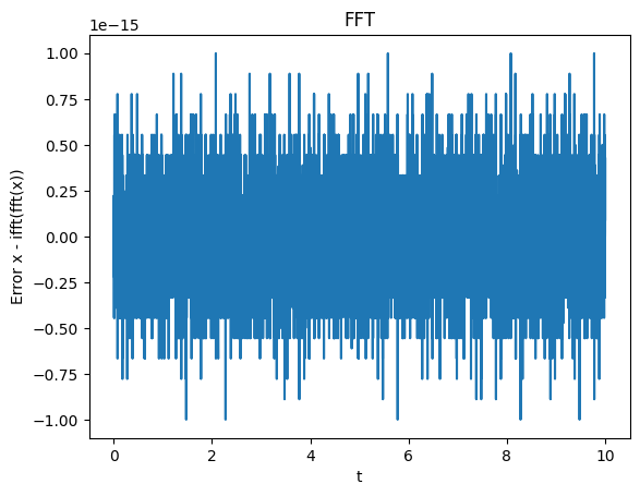
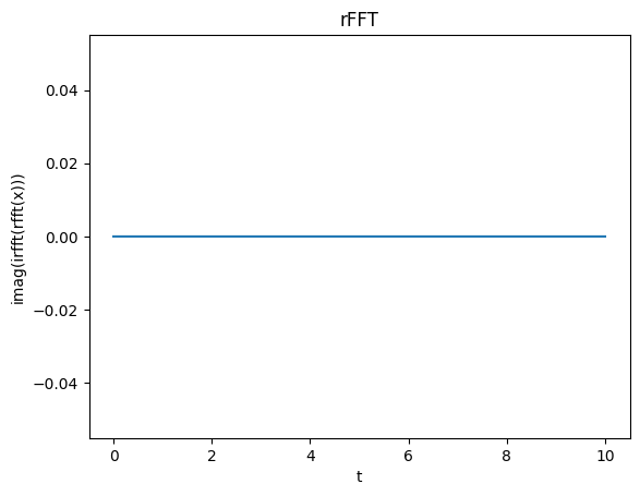
If the input array is real-valued (i.e. no complex numbers) then use rfft. Otherwise use fft. However, you can always use fft if you want but you might need to add extra steps to remove the complex noise from the results. E.g. if x is real-valued ifft(fft(x)) can be complex, due to numerical noise.
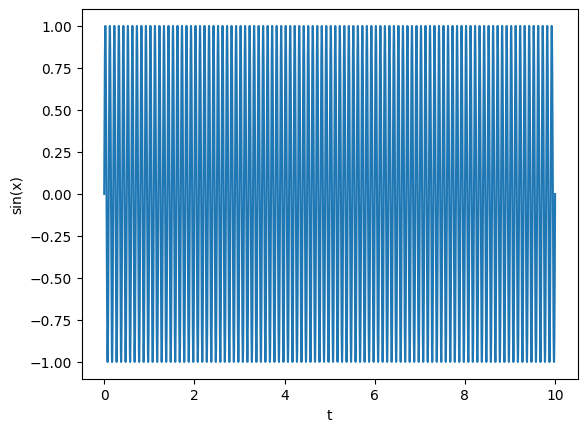
The test signal:
import numpy as np
import matplotlib.pyplot as plt

# Test signal
f: float = 10.0
t = np.linspace(0, 10, 10000)
x = np.sin(t * f * 2 * np.pi)

plt.plot(t, x)
plt.ylabel("sin(x)")
plt.xlabel("t")
plt.show()
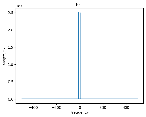
fft_result = np.fft.fft(x)
print(fft_result.shape) # -> (10000,)
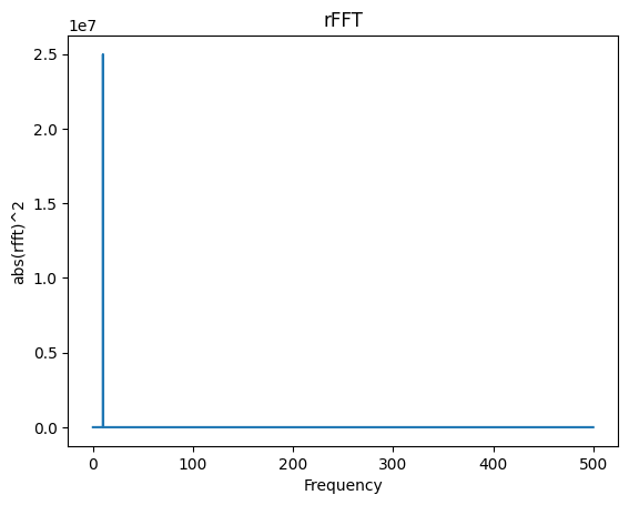
rfft_result = np.fft.rfft(x)
print(rfft_result.shape) # -> (5001,)
numpy.fft.fftfreq
fft.fftfreq(n, d=1.0)
Return the Discrete Fourier Transform sample frequencies.
The returned float array f contains the frequency bin centers in cycles per unit of the sample spacing (with zero at the start). For instance, if the sample spacing is in seconds, then the frequency unit is cycles/second.
Given a window length n and a sample spacing d:
f = [0, 1, ...,   n/2-1,     -n/2, ..., -1] / (d*n)   if n is even
f = [0, 1, ..., (n-1)/2, -(n-1)/2, ..., -1] / (d*n)   if n is odd
numpy.fft.rfftfreq
fft.rfftfreq(n, d=1.0)
Return the Discrete Fourier Transform sample frequencies (for usage with rfft, irfft).
The returned float array f contains the frequency bin centers in cycles per unit of the sample spacing (with zero at the start). For instance, if the sample spacing is in seconds, then the frequency unit is cycles/second.
Given a window length n and a sample spacing d:
f = [0, 1, ...,     n/2-1,     n/2] / (d*n)   if n is even
f = [0, 1, ..., (n-1)/2-1, (n-1)/2] / (d*n)   if n is odd
Unlike fftfreq (but like scipy.fftpack.rfftfreq) the Nyquist frequency component is considered to be positive.
Comparison (fftfreq)
The frequency axes:
dt = t[1] - t[0]
fft_freq = np.fft.fftfreq(x.shape[0],dt)
print(fft_freq.shape) # -> (10000,)

rfft_freq = np.fft.rfftfreq(x.shape[0],dt)
print(rfft_freq.shape) # -> (5001,)
plt.plot(fft_freq, np.abs(fft_result) ** 2)
plt.ylabel("abs(fft)^2")
plt.xlabel("Frequency")
plt.title("FFT")
plt.show()
plt.plot(rfft_freq, np.abs(rfft_result) ** 2)
plt.ylabel("abs(rfft)^2")
plt.xlabel("Frequency")
plt.title("rFFT")
plt.show()
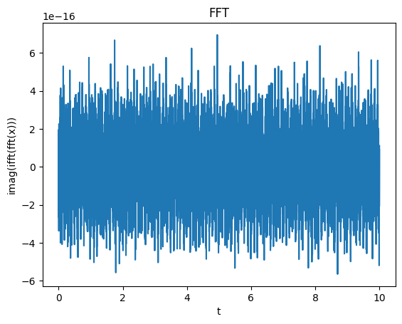
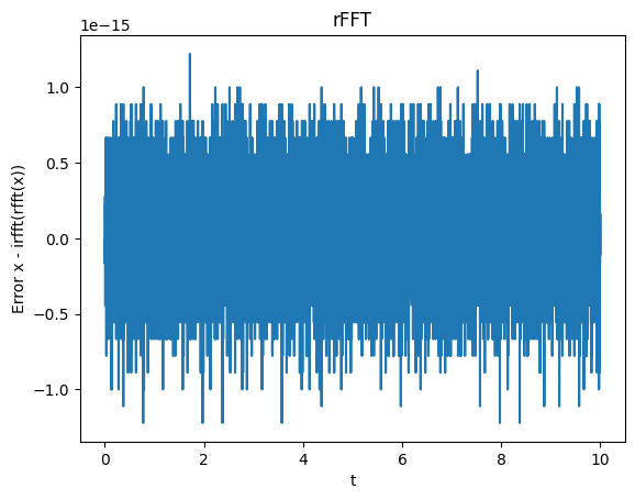
Comparison (ifft)
plt.plot(t, x - np.real(np.fft.ifft(fft_result)))
plt.ylabel("Error x - ifft(fft(x))")
plt.xlabel("t")
plt.title("FFT")
plt.show()
plt.plot(t, np.imag(np.fft.ifft(fft_result)))
plt.ylabel("imag(ifft(fft(x)))")
plt.xlabel("t")
plt.title("FFT")
plt.show()
plt.plot(t, x - np.real(np.fft.irfft(rfft_result)))
plt.ylabel("Error x - irfft(rfft(x))")
plt.xlabel("t")
plt.title("rFFT")
plt.show()
plt.plot(t, np.imag(np.fft.irfft(rfft_result)))
plt.ylabel("imag(irfft(rfft(x)))")
plt.xlabel("t")
plt.title("rFFT")
plt.show()
Discrete Fourier Transform (numpy.fft)
Standard FFTs
| fft(a[, n, axis, norm]) | Compute the one-dimensional discrete Fourier Transform. |
| ifft(a[, n, axis, norm]) | Compute the one-dimensional inverse discrete Fourier Transform. |
| fft2(a[, s, axes, norm]) | Compute the 2-dimensional discrete Fourier Transform. |
| ifft2(a[, s, axes, norm]) | Compute the 2-dimensional inverse discrete Fourier Transform. |
| fftn(a[, s, axes, norm]) | Compute the N-dimensional discrete Fourier Transform. |
| ifftn(a[, s, axes, norm]) | Compute the N-dimensional inverse discrete Fourier Transform. |
Real FFTs
| rfft(a[, n, axis, norm]) | Compute the one-dimensional discrete Fourier Transform for real input. |
| irfft(a[, n, axis, norm]) | Computes the inverse of rfft. |
| rfft2(a[, s, axes, norm]) | Compute the 2-dimensional FFT of a real array. |
| irfft2(a[, s, axes, norm]) | Computes the inverse of rfft2. |
| rfftn(a[, s, axes, norm]) | Compute the N-dimensional discrete Fourier Transform for real input. |
| irfftn(a[, s, axes, norm]) | Computes the inverse of rfftn. |
Hermitian FFTs
| hfft(a[, n, axis, norm]) | Compute the FFT of a signal that has Hermitian symmetry, i.e., a real spectrum. |
| ihfft(a[, n, axis, norm]) | Compute the inverse FFT of a signal that has Hermitian symmetry. |
Helper routines
| fftfreq(n[, d]) | Return the Discrete Fourier Transform sample frequencies. |
| rfftfreq(n[, d]) | Return the Discrete Fourier Transform sample frequencies (for usage with rfft, irfft). |
| fftshift(x[, axes]) | Shift the zero-frequency component to the center of the spectrum. |
| ifftshift(x[, axes]) | The inverse of fftshift. |
The source code is Open Source and can be found on GitHub.