Numpy – rfft and spectral power

Goal

We want to calculate a well behaved power spectral density from a 1 dimensional time series.

Generation of test data

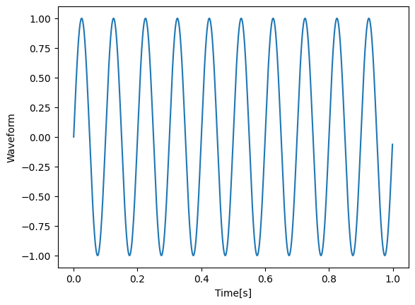
We will generate a sine wave with 10 Hz.

import numpy as np

time_series_length: int = 1000
dt: float = 1.0 / 1000.0  # time resolution is 1ms
sampling_frequency: float = 1.0 / dt
frequency_hz: float = 10.0
t: np.ndarray = np.arange(0, time_series_length) * dt
y: np.ndarray = np.sin(t * 2 * np.pi * frequency_hz)

Fourier transform with rfft

Since we deal with non-complex waveforms (i.e. only real values) we should use rfft. This is faster and uses less memory.

1 dimension


numpy.fft.rfft	Compute the one-dimensional discrete Fourier Transform for real input.
numpy.fft.irfft	Computes the inverse of rfft.
numpy.fft.rfftfreq	Return the Discrete Fourier Transform sample frequencies (for usage with rfft, irfft).

2 dimensions


numpy.fft.rfft2	Compute the 2-dimensional FFT of a real array.
numpy.fft.irfft2	Computes the inverse of rfft2.

N dimensions


numpy.fft.rfftn	Compute the N-dimensional discrete Fourier Transform for real input.
numpy.fft.irfftn	Computes the inverse of rfftn.

Since we deal with a 1 dimensional time series

y_fft: np.ndarray = np.fft.rfft(y)
frequency_axis: np.ndarray = np.fft.rfftfreq(y.shape[0]) * sampling_frequency

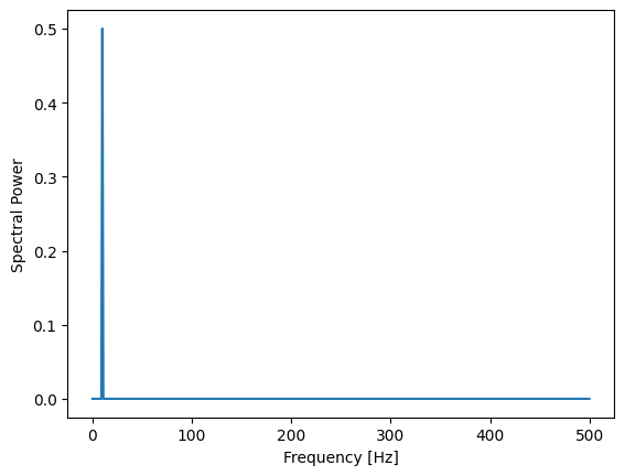
Calculating a normalized power spectral density

The goal is to produce a power spectral density that is compatible with the Parseval’s identity. Or in other words: the sum over the power spectrum without the zero frequency has the same value as the variance of the time series.

y_power: np.ndarray = (1 / (sampling_frequency * y.shape[0])) * np.abs(y_fft) ** 2
y_power[1:-1] *= 2

if frequency_axis[-1] != (sampling_frequency / 2.0):
    y_power[-1] *= 2

Check of the normalization:

print(y_power[1:].sum()/ (time_series_length * dt))  # -> 0.5
print(np.var(y))  # -> 0.5

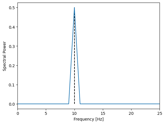
Or zoomed in:

The source code is Open Source and can be found on GitHub.