Symbolic Computation

Top

pip install sympy

Overview tutorials


Basic Operations
Printing
Simplification
Calculus
Solvers
Matrices

API Reference


Basics	Contains a description of operations for the basic modules. Subcategories include: absolute basics, manipulation, assumptions, functions, simplification, calculus, solvers, and some other subcategories.
Code Generation	Contains a description of methods for the generation of compilable and executable code.
Logic	Contains method details for the logic and sets modules.
Matrices	Discusses methods for the matrices, tensor and vector modules.
Number Theory	Documents methods for the Number theory module.
Physics	Contains documentation for Physics methods.
Utilities	Contains docstrings for methods of several utility modules. Subcategories include: Interactive, Parsing, Printing, Testing, Utilities.
Topics	Contains method docstrings for several modules. Subcategories include : Plotting, Polynomials, Geometry, Category Theory, Cryptography, Differential, Holonomic, Lie Algebra, and Stats.

Basics


Assumptions
Calculus
Combinatorics
Functions
Integrals
Series
Simplify
Solvers
abc
Algebras
Concrete
Core
Discrete
Numerical Evaluation
Numeric Computation
Term Rewriting

Some examples

Substitution

import sympy

x, y = sympy.symbols("x y")

expr = sympy.cos(x) + 1
z = expr.subs(x, y**2)
print(z) # -> cos(y**2) + 1

Derivatives

import sympy

x, y = sympy.symbols("x y")

y = sympy.diff(sympy.sin(x) * sympy.exp(x), x)
print(y) # -> exp(x)*sin(x) + exp(x)*cos(x)

Integrals

import sympy

x, y = sympy.symbols("x y")

y = sympy.integrate(sympy.cos(x), x)
print(y)  # -> sin(x)

(Taylor) Series Expansion

import sympy

x, y, z = sympy.symbols("x y z")
y = sympy.cos(x)
z = y.series(x, 0, 8) # around x = 0 , up order 7

print(z)  # -> 1 - x**2/2 + x**4/24 - x**6/720 + O(x**8)

simplify

import sympy

x, y, z = sympy.symbols("x y z")
y = sympy.simplify(sympy.sin(x) ** 2 + sympy.cos(x) ** 2)

print(y)  # -> 1

Solving Equations Algebraically

solveset(equation, variable=None, domain=S.Complexes)

Recall from the gotchas section of this tutorial that symbolic equations in SymPy are not represented by = or ==, but by Eq.

import sympy

x, y, z = sympy.symbols("x y z")

z = sympy.Eq(x, y)

Output:

\[x=y\]

import sympy

x, y, z = sympy.symbols("x y z")

y = sympy.Eq(x**2 - x, 0)
z = sympy.solveset(y, x)
print(z) # -> {0, 1}

Solving Differential Equations

import sympy

# Undefined functions
f = sympy.symbols("f", cls=sympy.Function)

x = sympy.symbols("x")

diffeq = sympy.Eq(f(x).diff(x, x) - 2 * f(x).diff(x) + f(x), sympy.sin(x))

print(diffeq)  # -> Eq(f(x) - 2*Derivative(f(x), x) + Derivative(f(x), (x, 2)), sin(x))

result = sympy.dsolve(diffeq, f(x))
print(result)  # -> Eq(f(x), (C1 + C2*x)*exp(x) + cos(x)/2)

Numerical Evaluation

import sympy

x, y = sympy.symbols("x y")

expr = sympy.cos(x) + 1
print(expr)  # -> cos(x) + 1
expr = expr.subs(x, 0.333 * sympy.pi)
print(expr)  # -> cos(0.333*pi) + 1
print(sympy.N(expr)) # -> 1.50090662536071

Plot your function

import sympy
import inspect
import numpy as np
import matplotlib.pyplot as plt

f = sympy.symbols("f", cls=sympy.Function)
x = sympy.symbols("x")
diffeq = sympy.Eq(f(x).diff(x, x) - 2 * f(x).diff(x) + f(x), sympy.sin(x))
result = sympy.dsolve(diffeq, f(x))

symbols = list(result.rhs.free_symbols)

f = sympy.lambdify(symbols, result.rhs, "numpy")


print("The arguments of the result:")
print(inspect.getfullargspec(f).args)
print("The source code behind f:")
print(inspect.getsource(f))

np_x = np.linspace(0, 2 * np.pi, 100)

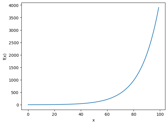
plt.plot(f(x=np_x, C1=1.0, C2=1.0))
plt.xlabel("x")
plt.ylabel("f(x)")
plt.show()

Assumptions about the symbols

C1 = sympy.symbols('C1', positive=True)


real=True	The symbol represents a real number.
positive=True	The symbol represents a positive number.
negative=True	The symbol represents a negative number.
integer=True	The symbol represents an integer.
prime=True	The symbol represents a prime number.
odd=True	The symbol represents an odd number.
even=True	The symbol represents an even number.

Limiting the range of a symbol

import sympy

x = sympy.symbols("x")
sympy.solve([x**2 - 1, x >= 0.5, x <= 3], x)

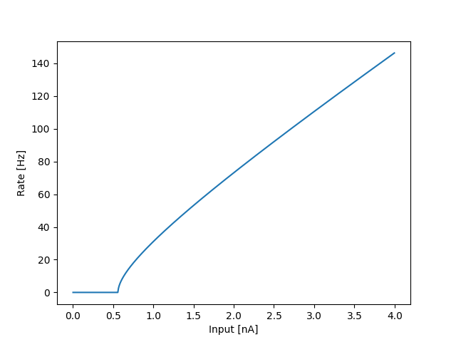
Example: Gain function of the quadratic integrate and fire neuron

import sympy
import numpy as np
import matplotlib.pyplot as plt

tau_value: float = 10e-3  # s
a0_value: float = 0.1e3  # V^-1
uc_value: float = -55.0e-3  # V
urest_value: float = -70.0e-3  # V
r_value: float = 10e6  # Ohm
uthr_value: float = -40e-3  # V

u = sympy.symbols("u", cls=sympy.Function, real=True)
urest, uc, uthr = sympy.symbols("urest uc uthr", real=True)
t, tau, a0, r, i = sympy.symbols("t tau a0 r i", real=True, positive=True)

c0, c1, c2 = sympy.symbols("c0 c1 c2", real=True)

diffeq_rhs = (a0 * (u(t) - urest) * (u(t) - uc) + r * i) / tau
diffeq_rhs = sympy.expand(diffeq_rhs)
diffeq_rhs = sympy.collect(diffeq_rhs, u(t))

c0_coeffs = diffeq_rhs.coeff(u(t), 0)
c1_coeffs = diffeq_rhs.coeff(u(t), 1)
c2_coeffs = diffeq_rhs.coeff(u(t), 2)

diffeq_rhs = diffeq_rhs.subs(c0_coeffs, c0)
diffeq_rhs = diffeq_rhs.subs(c1_coeffs, c1)
diffeq_rhs = diffeq_rhs.subs(c2_coeffs, c2)

diffeq = sympy.Eq(u(t).diff(t), diffeq_rhs)

solved_diffeq = sympy.dsolve(diffeq, u(t), ics={u(0): urest}, simplify=False)
solved_diffeq = solved_diffeq.subs(u(t), uthr)
solved_diffeq = sympy.simplify(solved_diffeq)

solved2_diffeq = sympy.solve(solved_diffeq, t)[0]

solved2_diffeq = solved2_diffeq.subs(c0, c0_coeffs)
solved2_diffeq = solved2_diffeq.subs(c1, c1_coeffs)
solved2_diffeq = solved2_diffeq.subs(c2, c2_coeffs)
solved2_diffeq = sympy.simplify(solved2_diffeq)

solved2_diffeq = solved2_diffeq.subs(tau, tau_value)
solved2_diffeq = solved2_diffeq.subs(a0, a0_value)
solved2_diffeq = solved2_diffeq.subs(uc, uc_value)
solved2_diffeq = solved2_diffeq.subs(urest, urest_value)
solved2_diffeq = solved2_diffeq.subs(r, r_value)
solved2_diffeq = solved2_diffeq.subs(uthr, uthr_value)
solved2_diffeq = sympy.simplify(solved2_diffeq)


print("The final function")
print(solved2_diffeq)
print()


thr_func = sympy.lambdify(i, solved2_diffeq, "numpy")

i = 4 * 1e-9 * np.arange(0, 1000, dtype=np.complex128) / 1000
z = thr_func(i)
z = 1.0 / z
z[z < 0] = 0
z = z.astype(dtype=np.float32)

plt.plot(i * 1e9, z)
plt.xlabel("Input [nA]")
plt.ylabel("Rate [Hz]")
plt.show()

The source code is Open Source and can be found on GitHub.